Table of Contents

Hyperparameter optimization is a crucial skill required to train a good machine learning model. Like feature engineering and feature selection, hyperparameter optimization is another step on the data-science workflow that requires and benefits from manual human intervention. This post will build up from defining hyperparameters and the different types that are out there and move on to the methods we have in our toolkit to try and select the best values for them.

What are Hyperparameters?¶

Unlike the parameters of a machine learning model, which are learned during the training process, hyperparamters cannot be learned from the training data. Model parameters are learned by trying to minimize a loss function while using an algorithm like gradient descent. A hyperparameter of the model is a variable whose value is set before the learning/training process begins. Furthermore, the parameters of a model decide how the data of fed into the algorithm needs to be transformed, while the hyperparameters govern the actual architecture of the model.

In simple terms, a hyperparameter is a value that cannot be automatically learned and will act like knobs on an equalizer that allow you set and dictate the mechanism and composition of the machine learning model you are trying to train.

Examples and types of Hyperparameters¶

The values of a hyperparameter are set when the model is initialized and before the training process begins. In sklearn, hyperparameters are passed in as arguments to the constructor of the model classes. Hyperparameters can be numerical (discrete or continuous) or categorical in nature.

Examples of Hyperparameters
Numerical

• The degree of polynomial features to use in a linear model
• The maximum depth of a decision tree
• The minimum number of samples required in a leaf node in a decision tree
• The number of trees to include in a random forest
• The number of layers to have in a neural network
• The learning rate of the gradient descent algorithm

Categorical

• The criterion to evaluate the best split at a node in a decision tree
• The type of regularization/penalty (L1, L2, Ridge) to use in a regression model
• The type of weight balancing to use in classification model with imbalanced data

Which hyperparameters should you tune?¶

Unfortunately, there isn't a one-size-fits-all magic formula when it comes to selecting how many hyperparameters or which ones you should tune. In general, if you have prior experience with the alogirthm you are using, you could have an idea about the effect of a hyperparameter on the model. Additionally, you could also find assistance in machine learning communities.

No matter how you choose which hyperparameters you'd like to tune, it's important to remember that each additional hyperparameter could significantly increase the number of trials and time required to successfully complete the tuning job.

How do you tune hyperparameters?¶

Mathematically, hyperparameter optimization can be represented as an equation:

In essence, this equation reads as find the value of x that minimizes the function f(x). In our case, x would be a hyperparameter and f(x) would be the objective function we are trying to minimize - such as the RMSE or Mean Absolute Error - on a validation set

In practice, this process looks like the following:

1. Define a model you wish to use. (RandomForest, Decision Trees, etc)
2. Define the range of possible values for all hyperparameters you wish to evaluate the model on. (Number of trees, Maximum depth of a tree, etc)
3. Define a method for sampling/selecting hyperparameter values (Exhuastive, Random, Sequential, etc)
4. Train the model for each unique combination of hyperparameter values
5. Define an evaluation criteria to judge each training iteration of the model with a validation set (RMSE or MAE)
6. Define a cross-validation method (k-fold, LOOCV, etc)

All the steps above, put together, constitute the objective function f(x) in our hyperparameter tuning, and the unique combination of hyperparameter values would make up the x

The challenge of hyperparameter tuning¶

As can be seen from the process listed above, in order to evaluate each set of hyperparameter values we need to train a model on the training data, make predictions on the validation data and then compute the validation metric. This is a time and computationally expensive process that may take minutes or days to complete depending on the size of the data and complexity of the model chosen (think ensembles or deep neural networks); making hyperparameter tuning an intractable problem.

Tuning Strategies¶

There are a number of methods one may implement to try and tune hyperparameters.

• Single Validation Set
• K-Fold Cross Validation
• Gird Search
• Random Search
• Bayesian Optimization
• Evolutionary Optimization
• Gradient Based Optimization

Load and split the data¶

Train a base model¶

Isolated Experimental Based Hyperparameter Optimization¶

Single Validation Set¶

A single validation set can be used to verify our values for hyperparameters by observing the impact on the loss function of our model on a validation/unseen set of data. The downside of this approach are plenty:
1) We only have one validation set, and depending on its size and how it was created, it might not serve as an accurate representation of real world data.
2) This method is manual and would be quite time consuming if we wanted to try several different hyperparameters and values

Tuning max_depth¶

Visualize the results¶

Important Note: In practice, you would never touch the test set when performing hyperparameter optimization and neither would you try to repeatedly predict on it. The reason I have showcased the Test_MSE is simply to illustrate what would have happened had we built a model with a particular hyperparameter value and to consolidate our understanding of the importance of validation / cross validation.

It appears that a max_depth of 3 results in the lowest Mean Squared Error of 10.999

Tuning min_samples_split¶

Visualize the results¶

Important Note: In practice, you would never touch the test set when performing hyperparameter optimization and neither would you try to repeatedly predict on it. The reason I have showcased the Test_MSE is simply to illustrate what would have happened had we built a model with a particular hyperparameter value and to consolidate our understanding of the importance of validation / cross validation.

It appears that a min_smaples_split of 4 results in the lowest Mean Squared Error of 10.683

k-Fold Cross Validation¶

In k-fold cross validation, the data is divided into "k" subsets. The model is then trained on k-1 subsets and the last susbet serves as the unseen validation set. This process is repeated k-times, with each of the k subsets having their turn to act as the unseen validation set, while the other k-1 subsets are put together to form the training set. The avearage score or loss of all k runs is calculated and used as a metric to make an informed selection for the hyperparameter values.

Unlike the single cross validation set, k-fold cross validation allows you to test your hyperparameter selection on multiple sets of unseen data. Hence, the resulting score or loss is more accurate indicator of how the model will perform on unseen data.

Tuning max_depth¶

Visualize the results¶

Important Note: In practice, you would never touch the test set when performing hyperparameter optimization and neither would you try to repeatedly predict on it. The reason I have showcased the Test_MSE is simply to illustrate what would have happened had we built a model with a particular hyperparameter value and to consolidate our understanding of the importance of validation / cross validation.

Tuning min_samples_split¶

Visualize the results¶

Important Note: In practice, you would never touch the test set when performing hyperparameter optimization and neither would you try to repeatedly predict on it. The reason I have showcased the Test_MSE is simply to illustrate what would have happened had we built a model with a particular hyperparameter value and to consolidate our understanding of the importance of validation / cross validation.

Tuning multiple hyperparatmeters simultaneously¶

In general, the avg_cross_validation MSE serves as a stronger indicator of the model's accuracy on unseen data given that it has been tested on more than a single validation set.

Important Note: In the MSE vs min_samlpes_split plot, we can see that MSE doesn't vary drastically with the increase in the min_samlpes_split. Hence, since the MSE is not a defining criteria, you should default to picking a hyperparameter value that results in a less complex model. In this case, we would pick a model with a larger min_samples split than a smaller one, as a smaller min_samples_split value would result in a more complex model. Remember, in practice you will never touch the test set and will not have it a line plotted for it.

In both the examples above, we only tried to optimize one hyperparameter at a time. However, it would be incorrect to combine the hyperparameter values from these isolated experiments and assume you have created the best model. This is because each hyperparameter was optimized in a mututally exclusive enviorment from the other. Hence, when we were optimizing for the min_samples_split, the max_depth of the model was the default value, and likewise when we were optimizing for the max_depth, the min_samples_split was the default value.

Let's try top optimize both these hyperparameters simultaneously. Since we have 9 different max_depths, and 22 unique min_samples_split sizes, finding the best hyperparameter values will require us to train the model 9x22 = 198 times. Once for each unique combination of hyperparameter values. Furthermore, we are performing a 5-fold cross validation, which will raise the total number of iterations of our objective function to 198x5 = 990.

Visualize the results¶

Important Note: In practice, you would never touch the test set when performing hyperparameter optimization and neither would you try to repeatedly predict on it. The reason I have showcased the Test_MSE is simply to illustrate what would have happened had we built a model with a particular hyperparameter value and to consolidate our understanding of the importance of validation / cross validation.

In essence, this was the manual process of performing grid search cross validation. In that we were given a hyperparmeter space with a set of values for each hyperparameter and we performed an exhaustive search across this space to find best results.

Grid Search¶

With Gird Search CV, a set of values is provided for each hyperparameter you wish to tune. The algorithm will then take the cartesian product of these sets and try evey unqiue combination of hyperparameters and return the values that result in the highest accuracy or lowest error.

The grid search algorithm is exhaustive in nature, in that it will try every combination of values in the hyperparameter space you provide. An advantage of the grid search algorithm is that it automates the process. However, as you can imagine, it is also time and computationally expensive.

Let's try to re-create the grid search we did above

As you can see, the values for the hyperparameterts suggested by the GridSearchCV algorithm are the same as our manual step above

You might notice a slight difference in test and validation MSE for the grid search algorithm. The reason for that is that the best_estimator_ in the GridSearchCV algorithm is trained on the entire "learning" data set, while in our manual step, it was trained only on "train" data set which excludes the test and validation data.

Random Search¶

Like Grid Search CV, Random Search CV also takes in a set of values for each hyperparameter you wish to tune. However, the major difference being that unlike GridSearchCV that exhaustively tries every combination of hyperparameter values, RandomSearchCV randomly selects values from the hyperparameter space you provided.

While this random selection does not guarantee that the algorithm will select the best hyperparameters for your model, it does come with a significant boost in speed.

Furthermore, with the 9 different max_depths, and 22 unique min_samples_split sizes, we have 9x22 = 198 unique combinations of hyperparameters (the cartesian product of the two sets). However, the Random Search CV has a hyperparameter of its own called "n_iter" that allows us to dictate how many of 198 combinations should be randomly selected. We will set this value to 20 below, and have a 5-fold cross validation whihc result in 100 evaluations of our objective function.

As we can see, RandomSearch CV did not give us the lower validation or Test MSE. However, the time it was able to complete the task in a fifth of the time and provided a result that was decently comparable to GridSearch CV.

Sequential Model Based Optimization (SMBO)¶

If you hadn't noticed already, all of the methods listed above had one thing in common; each of them ran independent experiments of training and evaluating a model for each combination of hyperparameter values. While the GridSearchCV and RandomSearchCV algorithms do help us narrow in on the best of hyperparameter values from the options they try, they fail to carry over any information from each iteration to the next.

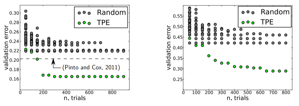
Consider the image above, which is taken from Making a Science of Model Search: Hyperparameter Optimization in Hundreds of Dimensions for Vision Architectures. These figures compare the validation error for hyperparameter optimization of an image classification neural network with random search in gray and an Sequential Model Based Optimization (SMBO) in green. The image clearly exhibits the prowess of the SMBO method.

First, a smaller validation error is achieved, which signifies a better model, and second it does so in a smaller number of trials, hence saving time.

This is fundamentally a big disadvantage of the isolated experimental based hyperparameter optimization techniques. Since GridSearchCV and RandomSearchCV are completely uninformed by their past evaluations, they often spend a significant amount of time evaluating "bad" hyperparameters.

Bayesian Optimization¶

In contrast to the experimental based techniques, Bayesian optimization is a sequential model based optimization technique for evaluating the best hyperparameters. The Bayesian approach keeps track of past evaluations results and uses it to build a probabilistic model mapping hyperparameters to a probability of a score on the objective function.

P(Score|Hyperparameters)

Let's dive a little depper into the workings of the Bayesian approach. There are two definitions in particular that we need to be aware of with Bayesian optimization or any SMBO technique in general.

Surrogate Model¶

Recollect that one of the challenges facing hyperparameter optimization is the duration it takes to evaluate the performance of a model due to the need to retrain and reevaluate the model for each combination of hyperparameter values. This process is what we have been referring to as our objective function.

One of the big performance improvements in the Bayesian optimization comes as a result of adopting a Surrogate Model. The surrogate model is a probabilistic model that is much easier to evaluate than our true objective function and hence yields a solution in a drastically shorter duration of time.

There are several surrogate models that you can choose from:

• Gaussian Processes
• Tree Parzen Estimators
• Random Forest Regressors

Acquisition or Selection Function¶

The Acquisition function helps select the next set of hyperparameter values to pass into the surrogate model. There are 3 acquisition functions that I have come across:

• Upper Confidence Bound
• Probability of Improvement
• Expected Improvement (Most Common)

How does it work?¶

With these two definitions under our belt, we are now ready to understand the process used in Bayesian Optimization.

1. Define a domain of hyperparameters over which to search (for example max_depth = [1,2,3,4,5] and min_samples_split = [2,3,4,5,6]).
2. Define an objective function which takes in hyperparameters as inputs, trains a machine learning model and outputs a score such as RMSE or Mean absolute error that we want to minimize (or maximize).
3. Define a surrogate probability model that aims to replicate the true objective function defined in step 2.
4. Define an Acquisition or Selection function for evaluating which hyperparameters perform best on the surrogate model defined in step 3.
5. Use the Acquisition function defined in step 4 to select the best performing hyperparamters.
6. Select the hypeparameters that perform best on the surrogate model and apply/pass them to the true objective function to get a score.
7. Use the score given hyperparameters (score | hyperparameter) from step 6 to update the surrogate model
8. Repeat steps 5,6 and 7 until you reach the maximum iterations or time.

The main idea in the above process is to spend a little more time exploring potential hyperparameter values and spend a lot less time evaluating the true objective function. In practice, the extra time spent exploring is inconsequential to the time you would spend evaluating the objective function. Hence, the net effect is an algorithm that learns from every iteration, makes more informed decisions about which hyperparameter value(s) to try next and saves a lot of time that would have otherwise been wasted evaluating bad hyperparameters.

Visualizing Bayesian Optimization

Example of Bayesian Optimization¶